Scope view
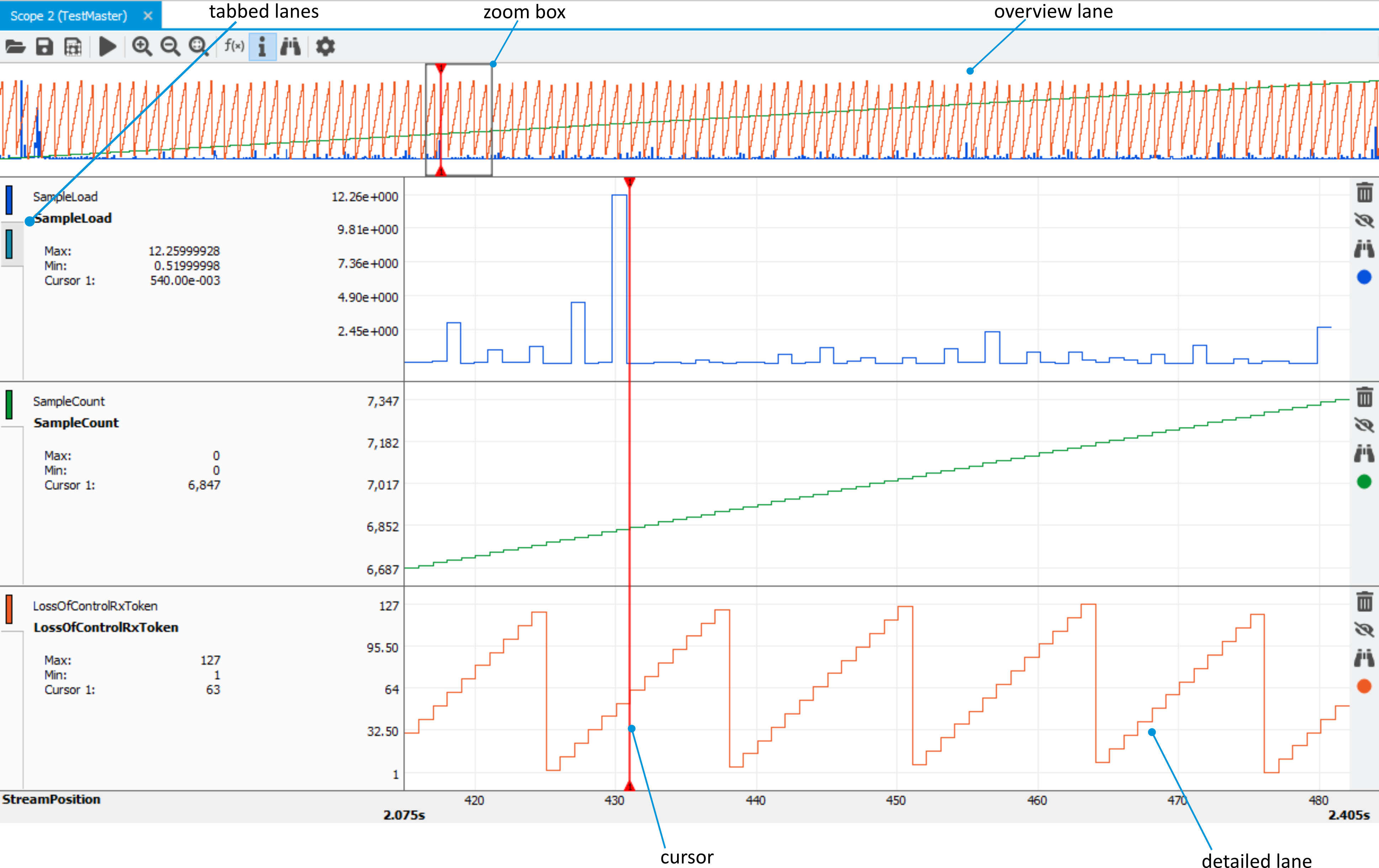
A Scope view plots signals values (see Scope view). The view can be added by clicking . Alternatively, a Scope view can be opened by right-clicking the controller in the Network explorer and selecting from the context menu. Each scope window is associated with a single controller, the controller related to the Scope view is displayed in the window title. Multiple scopes can be opened at the same time.
The annotated key elements are described in the sections below.
Scope view
The main functions of the Scope view can be controlled via the toolbar (see Scope view toolbar).
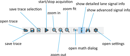
Scope view toolbar
Scope settings
Before starting an acquisition, the acquisition settings have to be configured. The settings are categorized into three tabs, General, Signals and Triggering settings.
General
General settings consist of all settings regarding the acquisition and subsequent plotting of the signals (see General settings dialog).
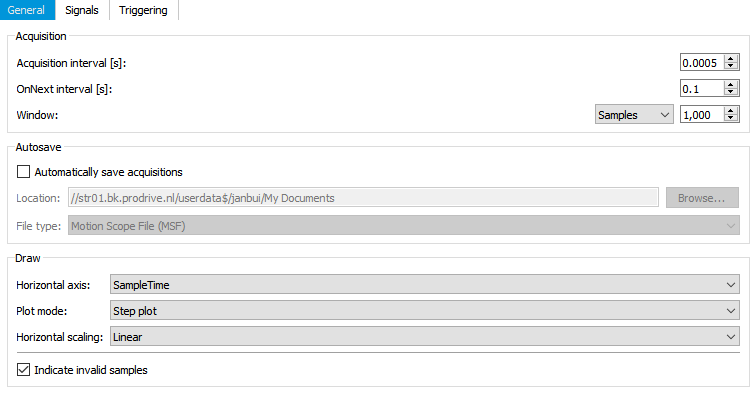
General settings dialog
Acquisition window
The acquisition window defines the number of samples, which are kept before old samples are thrown away. By default, this is used to limit the memory used by the Scope view.
Autosave
If automatic saving is enabled, all samples are saved to a file with the selected format as they are acquired. A new file is created each time an acquisition is started. The file name contains the name of the Scope view that started the acquisition and the time at which it was started.
This feature can be used in combination with the acquisition window for long-running acquisitions. All samples are stored in a file, but only the most recent samples are kept in memory, limiting memory usage.
Draw
The “Draw” heading contains settings that determine the way acquired samples are drawn. These settings apply to all lanes.
Horizontal axis: Determines which signal is used as the horizontal axis.
Plot mode: Determines the method by which samples are drawn. Possible options are: step plot, scatter plot and line plot.
Horizontal scaling: Determines how the horizontal axis is scaled, linearly or logarithmically.
Indicate invalid samples: Determines whether invalid samples are indicated by shading the invalid region in the lane. Missing samples are shaded grey, samples with infinite values are shaded red and samples with not-a-number (NaN) values are shaded yellow.
Signals
Signals can be added to the scope in two different ways. First, by dragging signals directly from the Network explorer to the scope view. Alternatively, signals can be dragged to the Signals tab shown in Signal settings dialog.
All signals in the scope are displayed in this Signals tab. In the tab, multiple signals can be selected at the same time. Using the toolbar shown in Signal settings dialog, actions can be applied to the selected signals. The actions that are supported are listed below.
Alter the selected signals sampling interval (Ctrl + I).
Merge selected signals (Ctrl + M).
Unmerge selected signals (Ctrl + U).
Toggle selected signals visibility (Ctrl + H).
Delete selected signals (Del).
Add a math signal (Ctrl + F).
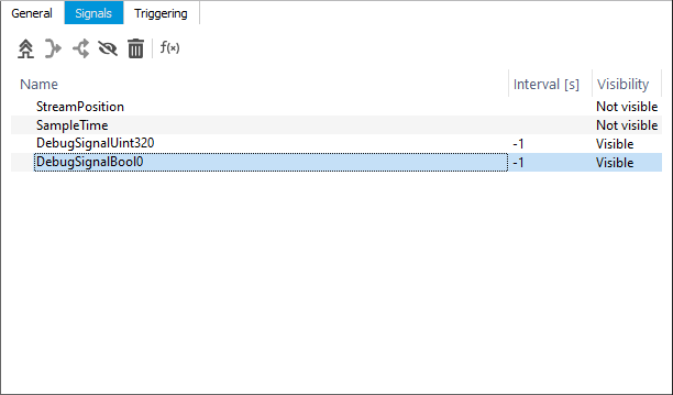
Signal settings dialog
Triggering
Trigger settings dialog. shows an example of a trigger configuration. A start and stop condition have been defined as well as a pre and post-sample time.
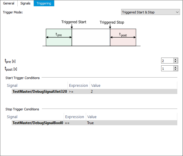
Trigger settings dialog.
If the acquisition triggers have been set, they will automatically be applied when the acquisition is started. Acquisition trigger example using configurations shown in trigger_settings. displays the resulting acquisition which indicates the behavior of the previous configuration.
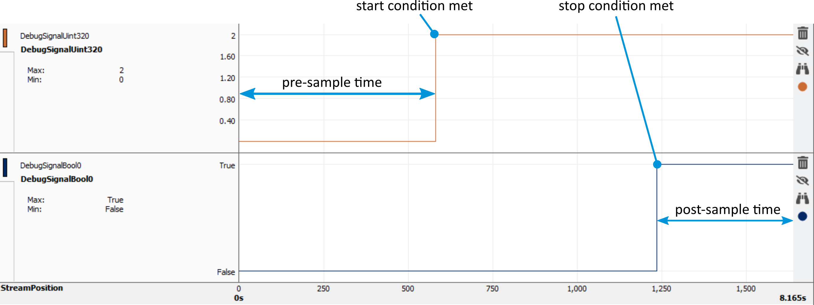
Acquisition trigger example using configurations shown in Trigger settings dialog..
Start, stop and save an acquisition
An acquisition is started by clicking on the Play button. Once an acquisition is started, it runs until the user stops it. Alternatively, an acquisition can be started or stopped by triggered acquisition as discussed in Triggering section.
An acquisition can be saved as .msf or .csv file.
To save a selection of an acquisition, select the desired interval in the toolbar (see Zooming section) and click .
A previously saved acquisition can be opened by clicking Open acquisition and selecting the desired file, or by dragging and dropping the file into the Scope view.
Overview lane
The overview lanes combine the detailed lanes into one overview. The overview lane can show all acquired signals (signals visibility in the overview can be changed with the Show in overview button.
Detailed lane
A detailed lane plots an acquired signal. Lanes can be re-oder by dragging them with the tab. It is possible to merge two lanes by drag and dropping a lane onto another lane. The lanes are tabbed, as shown in Scope view.

Lane toolbar
- The four buttons (see Lane toolbar) to the right of each lane are used to (from top to bottom):
Delete the signal in the lane.
Hide the lane.
Open the Signal advanced information view.
Change the color of the signal in the lane.
When a signal is hidden, it will not be shown in the scope. Hidden signals are still displayed in the Signals tab and can be toggled to visible.
Note
When saving an acquisition using Save selection, hidden lanes are not saved.
Horizontal axis
The horizontal axis is shared over all the detailed lanes. The current time window is shown below the horizontal axis values (see Horizontal axis).
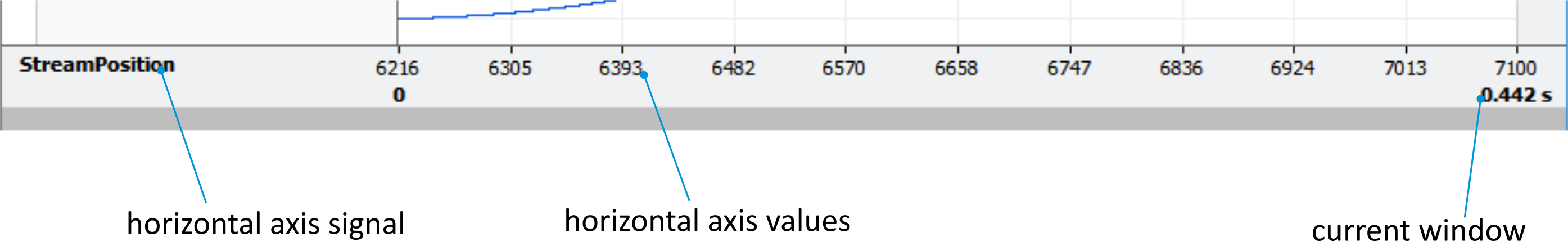
Horizontal axis
The horizontal axis is always associated with an acquired signal (shown in the left label). The signals (StreamPosition and SampleTime are acquired by default. To change the horizontal axis, open the settings tab shown in General and change the horizontal axis selection box.
Vertical axis
By default, the vertical axes scaling is performed automatically. However, it is also possible to set the vertical axis limits manually. To open the vertical axis dialog right-click on the lane and click . To configure the manual scale, uncheck Automatic scaling, fill in the desired limits and press on OK (see Vertical scale dialog).
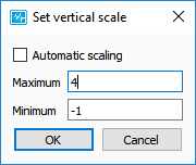
Vertical scale dialog
A single vertical axis is shown for all signals in a merged lane. By default, this vertical axis shows a combined scale of all the signals. To associate the vertical axis with a specific signal, right-click on the lane and uncheck Combine axes. Now the vertical axis will scale according to the signal selected in the tab.
Lane context menu
Some draw settings can be changed by right-clicking that lane, which opens the lane context menu.
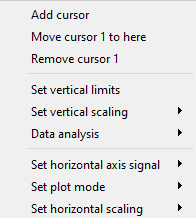
Lane context menu.
The first group of actions in this menu relates to cursors, the second group contains actions that relate to draw settings that apply only to the lane on which the context menu was opened and the last group contains settings that apply to all lanes.
Cursor
A cursor shows the value of a specific sample. To add a cursor, right-click in the lane and select . If two cursors are added, their relative position can be fixed by clicking in the context menu (see Scope cursors).
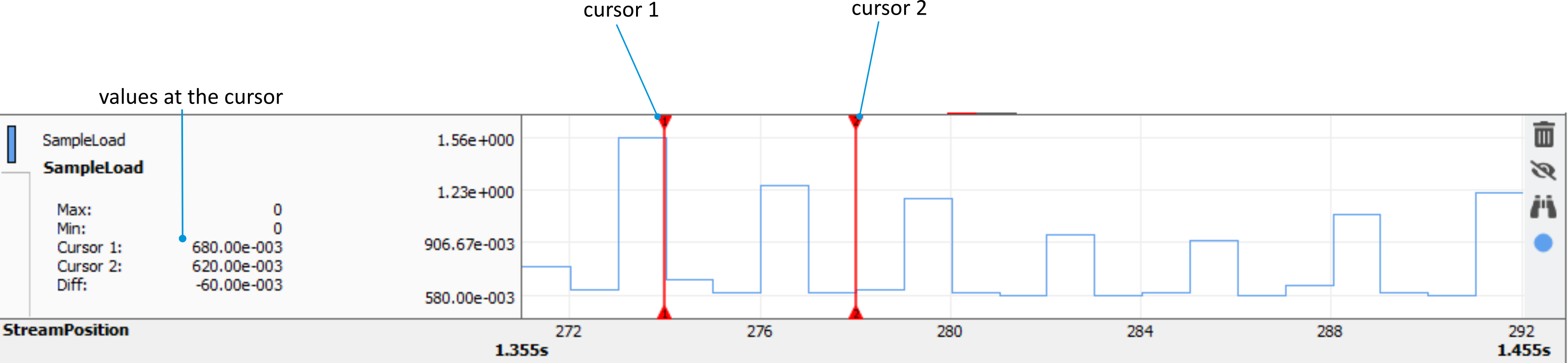
Scope cursors
Zooming
It is possible to zoom in and zoom out on detailed lanes by using the ![]() ,
, ![]() and
and ![]() icons in the toolbar (see Scope view toolbar).
Alternatively, clicking and dragging the mouse over the overview or detailed lane will create a zoombox in the selected area.
The associated zoom is shown as a zoom box in the signal overview lane.
Alternatively, one could create a zoom box by making a selection in the signal overview lane (see Zoom box in signal overview).
icons in the toolbar (see Scope view toolbar).
Alternatively, clicking and dragging the mouse over the overview or detailed lane will create a zoombox in the selected area.
The associated zoom is shown as a zoom box in the signal overview lane.
Alternatively, one could create a zoom box by making a selection in the signal overview lane (see Zoom box in signal overview).
Zoom box in signal overview
The zoom box size (zoom in or zoom out) can be changed by dragging the zoom box edge (or press Ctrl-Scroll). The position of the zoom box can be changed by either dragging it, pressing the LeftArrow and RightArrow keys, or using Shift-ScrollWheel.
Math dialog
To perform mathematical operations on acquired signals, open the Math dialog by clicking on the ![]() icon (see Math dialog).
A math expression can be applied to all signals.
Math signals can be added both before or after the acquisition and are updated during an acquisition.
icon (see Math dialog).
A math expression can be applied to all signals.
Math signals can be added both before or after the acquisition and are updated during an acquisition.
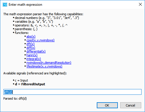
Math dialog
Aside from the regular mathematical operations, the following functions are available when using the math dialog:
abs(x): is the absolute value of the (real) elements in x.
diff(x): is the difference between elements in x, where the first output value equals zero.
differential(x): is the first order derivative of the (real) elements in x, where the first output value equals zero.
integral(x): is the integral of the (real) elements in x.
dft(x): is the discrete Fourier transform (DFT) of vector x. Output is normalized single sided frequency spectrum.
hann(x): applies one single Hanning window to vector x (begin and end will be zero).
nwindows(in, demandResolution): returns the number of windows (50% overlap) to be applied on vector with dimensions of in to achieve the demandResolution when used in combination with tfestimate() or cpsd() function.
cpsd(x, y, nwindows): calculates Pxy which is the Cross Power Spectral Density (CPSD) of time domain vectors x and y, using the Welch averaging method. nwindows must be a positive odd value for the number of (Hann) windows that are used with 50% overlap. When nwindows is 0, one rectangular window (no averaging) is done. Output is of complex type.
tfestimate(x, y, nwindows): estimates the Transfer Function with input x and output y, using the Welch averaging method. nwindows must be a positive odd value for the number of (Hann) windows that are used with 50% overlap. When nwindows is 0, one rectangular window (no averaging) is done. Output is normalized single sided frequency spectrum.
Data analysis dialog
The data analysis dialog can be used to perform certain mathematical operations in a more convenient way. It can be opened from the lane context menu (see Lane context menu.).
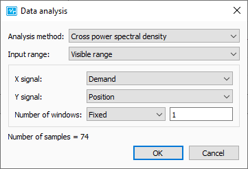
Data analysis dialog.
The dialog is used to configure the data source for the desired analysis operation. By default, the lane on which the analysis dialog was opened is used. After pressing “Ok”, the result of the analysis is opened in a new Scope view window.
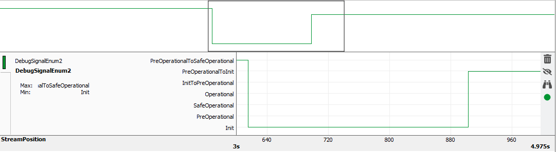
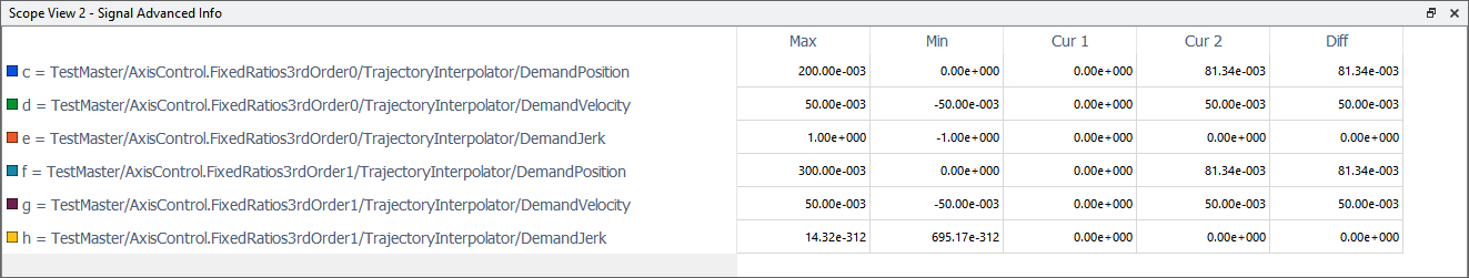
Signal advanced information view
The  icon opens the Signal advanced info view (see Advanced signal information view).
This view lists the minimum and maximum value of each signal in the acquisition, as well as the signal values at cursor positions (if applicable).
This can also be done for a single lane, by pressing the Signal advanced information in the detailed lane, shown in Lane toolbar.
icon opens the Signal advanced info view (see Advanced signal information view).
This view lists the minimum and maximum value of each signal in the acquisition, as well as the signal values at cursor positions (if applicable).
This can also be done for a single lane, by pressing the Signal advanced information in the detailed lane, shown in Lane toolbar.
Advanced signal information view